Transparent overlays of split-screen grid co-ordinates using ggplot2
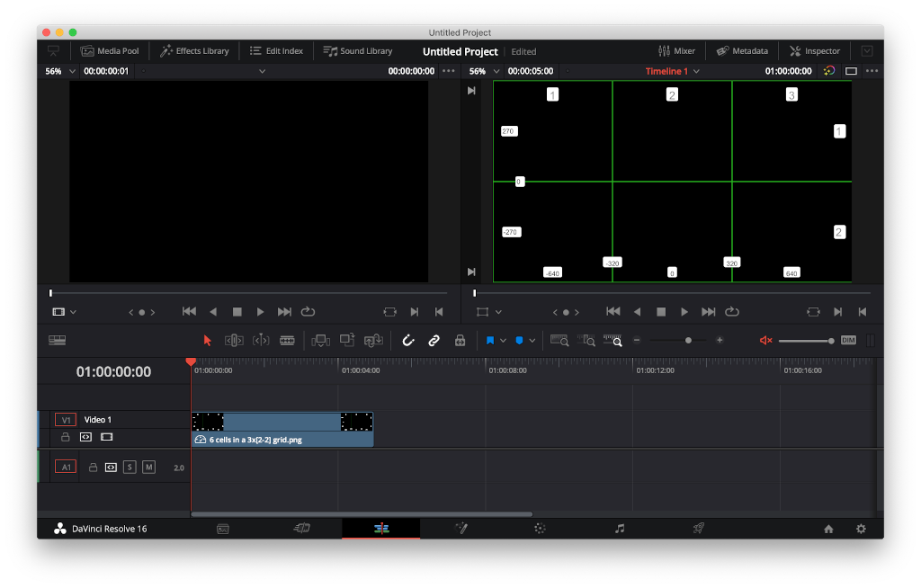
When editing split-screen video to create a regular grid layout in the free video-editing application DaVinci Resolve, I’ve found it helpful to have a transparent image file labelled with the co-ordinates of each ‘cell’.
I can drop this on top of the timeline and it helps me to position each video correctly.
I’ve written some R functions which use ggplot2 to plot any grid layout at any resolution and calculate the relevant co-ordinates. I’ve then used these to generate image files for a variety of 1080p HD grid layouts. You could use the same functions to produce different layouts or use a different resolution, or to change the offset so that for example the origin is in the bottom-left corner instead of the centre.
TL;DR – you may prefer to just download a ZIP file of images for 1080p grids up to 48 cells with a maximum of 8 rows or columns, ignoring any grids for which the cells have aspect ratios more extreme than 16:9 or 9:16.
If you’re interested in the R code used to generate these grids, keep reading!
First we load the tidyverse and some other useful packages: conflicted and glue.
library(conflicted)
library(glue)
suppressPackageStartupMessages(library(tidyverse))

suppressMessages(conflict_prefer("filter", "dplyr"))
If we’re deciding what grid layout to use, we might want to preview some layouts. The function below creates a preview plot of a single grid for a single resolution.
The function arguments specify the number of columns and rows, the x-
and y-resolution, and the desired title and subtitle of the plot. They
also specify the offset for co-ordinates – by default the origin is in
the centre to match DaVinci
Resolve, so
the offset is half the x- or y-resolution. However if you wanted the
origin to be in the bottom left, you could set the x_offset and
y_offset arguments to 0.
get_single_preview_grid_ggplot <- function(
  cols, rows, x_res, y_res, x_offset = -0.5 * x_res, y_offset = -0.5 * y_res,
  title = NULL, subtitle = NULL
) {
  x_lines <- seq(0, x_res, x_res / cols) + x_offset
  y_lines <- seq(0, y_res, y_res / rows) + y_offset
  x_breaks <- seq(0, x_res, 0.5 * (x_res / cols)) + x_offset
  y_breaks <- seq(0, y_res, 0.5 * (y_res / rows)) + y_offset
  x_label_positions <- head(x_lines, -1) + (0.5 * (x_res / cols))
  y_label_positions <- head(y_lines, -1) + (0.5 * (y_res / rows))

  p <- ggplot() +
    # vertical grid lines
    geom_segment(
      aes(x = x_lines, xend = x_lines),
      y = y_offset,
      yend = y_res + y_offset
    ) +
    # horizontal grid lines
    geom_segment(
      aes(y = y_lines, yend = y_lines),
      x = x_offset,
      xend = x_res + x_offset
    ) +
    # column numbers along top
    geom_text(
      aes(label = seq(1, cols, 1)),
      x = x_label_positions,
      y = y_res + y_offset,
      vjust = 1.5,
      size = 5,
      colour = "gray60"
    ) +
    # row numbers along right-hand side
    geom_text(
      aes(label = seq(rows, 1, -1)),
      y = y_label_positions,
      x = x_res + x_offset,
      hjust = 1.5,
      size = 5,
      colour = "gray60"
    ) +
    scale_x_continuous(
      breaks = x_breaks,
      guide = guide_axis(n.dodge = 2),
      labels = function(x) round(x, digits = 1)
    ) +
    scale_y_continuous(
      breaks = y_breaks,
      guide = guide_axis(n.dodge = 2),
      labels = function(x) round(x, digits = 1)
    ) +
    labs(title = title, subtitle = subtitle) +
    theme_void() +
    theme(axis.text = element_text(size = 11))

  p
}
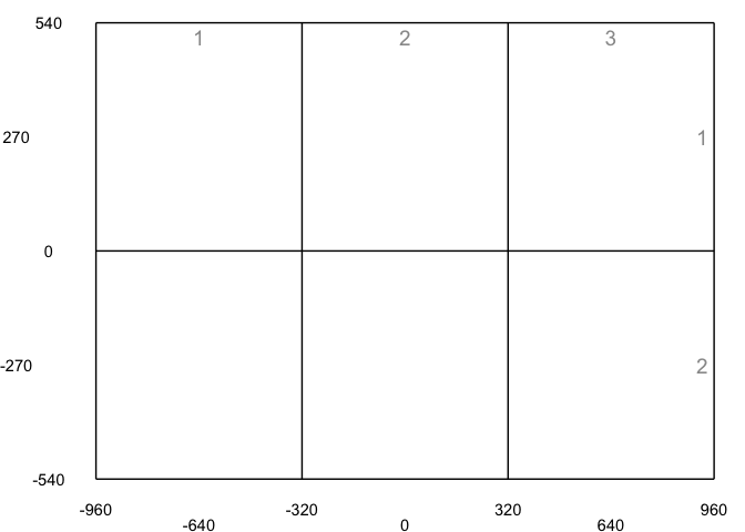
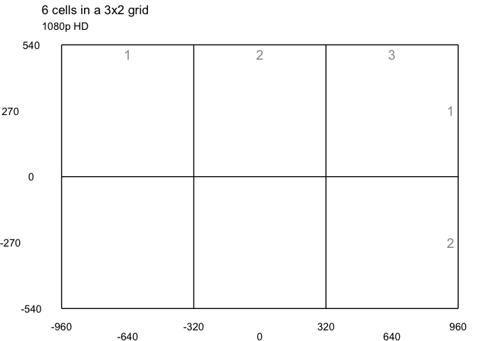
Here’s an example of using the function above to create a 3x2 grid with
1080p HD co-ordinates. Notice how the n.dodge argument of the
guide_axis
function, new
in ggplot 3.3.0,
has been used to alternate the position of the axis labels. This is
particularly useful when we have a much larger grid layout to prevent
the labels from overlapping.
get_single_preview_grid_ggplot(3, 2, 1920, 1080)
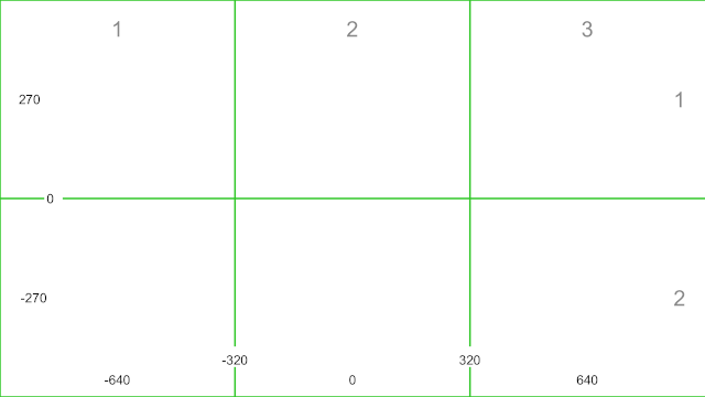
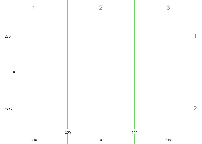
Like the function above, the function below creates a single plot for a particular grid layout. However this time there are no borders so that we can export the plot as an image to be overlaid on the video-editing timeline.
get_single_overlay_grid_ggplot <- function(
  cols, rows, x_res, y_res, x_offset = -0.5 * x_res, y_offset = -0.5 * y_res
) {
  x_lines <- seq(0, x_res, x_res / cols) + x_offset
  y_lines <- seq(0, y_res, y_res / rows) + y_offset
  x_pixels <- (seq(0, x_res, 0.5 * (x_res / cols)) + x_offset) %>%
    # remove first and last
    head(-1) %>%
    tail(-1) %>%
    round(digits = 1)
  y_pixels <- (seq(0, y_res, 0.5 * (y_res / rows)) + y_offset) %>%
    # remove first and last
    head(-1) %>%
    tail(-1) %>%
    round(digits = 1)
  x_label_positions <- head(x_lines, -1) + (0.5 * (x_res / cols))
  y_label_positions <- head(y_lines, -1) + (0.5 * (y_res / rows))

  p <- ggplot() +
    # vertical grid lines
    geom_segment(
      aes(x = x_lines, xend = x_lines),
      y = y_offset,
      yend = y_res + y_offset,
      colour = "limegreen"
    ) +
    # horizontal grid lines
    geom_segment(
      aes(y = y_lines, yend = y_lines),
      x = x_offset,
      xend = x_res + x_offset,
      colour = "limegreen"
    ) +
    # column numbers along top
    geom_label(
      aes(label = seq(1, cols, 1)),
      x = x_label_positions,
      y = y_res + y_offset,
      vjust = 1.5,
      size = 5,
      colour = "gray60",
      label.size = 0 # no border
    ) +
    # row numbers along right-hand side
    geom_label(
      aes(label = seq(rows, 1, -1)),
      y = y_label_positions,
      x = x_res + x_offset,
      hjust = 1.5,
      size = 5,
      colour = "gray60",
      label.size = 0 # no border
    ) +
    # pixel numbers along bottom
    geom_label(
      aes(
        label = x_pixels,
        x = x_pixels,
        # alternating heights
        y = rep_len(c(y_offset, y_offset + (y_res / 20)), length(x_pixels)),
      ),
      size = 3,
      vjust = -0.5,
      label.size = 0 # no border
    ) +
    # pixel numbers along left-hand side
    geom_label(
      aes(
        label = y_pixels,
        y = y_pixels,
        # alternating positions
        x = rep_len(c(x_offset, x_offset + (x_res / 20)), length(y_pixels)),
      ),
      size = 3,
      hjust = -0.5,
      label.size = 0 # no border
    ) +
    # remove axis expansion and theme elements to get just the plot panel
    scale_x_continuous(expand = c(0, 0)) +
    scale_y_continuous(expand = c(0, 0)) +
    theme_void()

  p
}
Here’s an example of using the function above to create a 3x2 grid with
1080p HD co-ordinates. Notice how the combination of theme_void and
removing the axis expansion using scale_*_continuous has removed any
borders from around the plot.
get_single_overlay_grid_ggplot(3, 2, 1920, 1080)
Creating single grids using a function is great, but we can iterate these functions to easily create multiple grid layouts. The code below defines a new function to create a table of possible grid layouts that we might want to use. We store preview and overlay plots generated by the functions above in two list columns as part of the table.
get_multiple_grids <- function(
  max_cols, max_rows, max_cells = Inf, x_res = 1920, y_res = 1080,
  x_offset = -0.5 * x_res, y_offset = -0.5 * y_res,
  subtitle = NULL
) {
  # create a table with all possible combinations of rows and columns
  grids <- expand_grid(
    cols = 2:max_cols,
    rows = 2:max_rows
  ) %>%
    # add some statistics about each grid layout
    mutate(
      cells = cols * rows,
      width = x_res / cols,
      height = y_res / rows,
      aspect_ratio = width / height
    ) %>%
    filter(cells <= max_cells) %>%
    mutate(
      # create a fancy title for each plot
      title = glue("{cells} cells in a {cols}x{rows} grid"),
      # run preview plot function for each combination of colunmns and rows
      preview_plot = pmap(
        list(cols, rows, x_res, y_res, x_offset, y_offset, title),
        ~ get_single_preview_grid_ggplot(
          ..1, ..2, ..3, ..4, ..5, ..6, ..7, subtitle
        )
      ),
      # run overlay plot function for each combination of columns and rows
      overlay_plot = pmap(
        list(cols, rows, x_res, y_res, x_offset, y_offset),
        get_single_overlay_grid_ggplot
      )
    )

  grids
}
Here we generate multiple grid layouts up to a maximum of 3 columns or rows. Notice how the plots are stored in the final two columns of the table. We’ll retrieve these later.
get_multiple_grids(max_cols = 3, max_rows = 3)
## # A tibble: 4 x 9
##    cols  rows cells width height aspect_ratio title    preview_plot overlay_plot
##   <int> <int> <int> <dbl>  <dbl>        <dbl> <glue>   <list>       <list>
## 1     2     2     4   960    540         1.78 4 cells… <gg>         <gg>
## 2     2     3     6   960    360         2.67 6 cells… <gg>         <gg>
## 3     3     2     6   640    540         1.19 6 cells… <gg>         <gg>
## 4     3     3     9   640    360         1.78 9 cells… <gg>         <gg>
Let’s use the get_multiple_grids function defined above to generate
layouts up to a maximum of 16 cells. We’ll filter out any extreme aspect
ratios (i.e. wider than 16:9 or taller than 9:16) using the between
function, even if
they’re the only option for a particular number of cells. We’ll also
choose a maximum of one layout for each particular number of cells: for
this example, the one that most closely matches a square aspect ratio.
chosen_grids <- get_multiple_grids(
  max_cols = 8, max_rows = 8, max_cells = 16, subtitle = "1080p HD"
) %>%
  filter(between(aspect_ratio, 9/16, 16/9)) %>%
  arrange(cells, cols)

# change to FALSE to skip choosing the grid that most closely matches a
# desired aspect ratio for each particular number of cells
if(TRUE) {
  desired_aspect_ratio <- 1/1 # i.e. a square

  chosen_grids <- chosen_grids %>%
    mutate(
      # using abs and log means that aspect ratios that are similarly distant from
      # the desired ratio will get the same score e.g. if desired aspect ratio = 1
      # i.e. a square, the ratios 3:2 and 2:3 will produce a score of 0.405
      aspect_ratio_difference = abs(log(aspect_ratio / desired_aspect_ratio))
    ) %>%
    group_by(cells) %>%
    top_n(-1, aspect_ratio_difference)
}
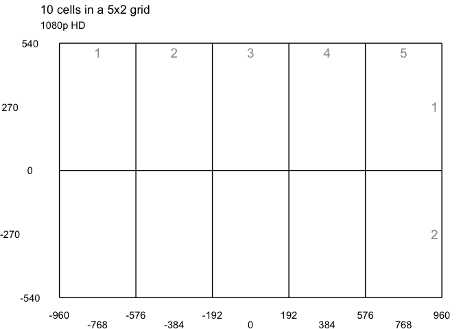
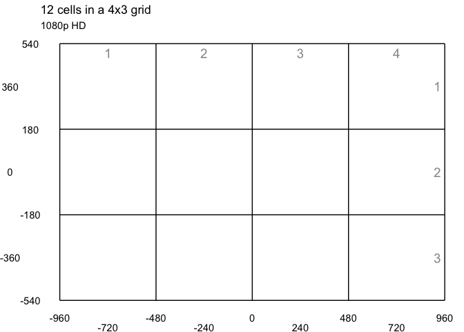
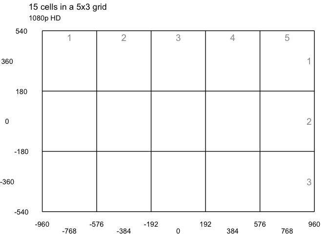
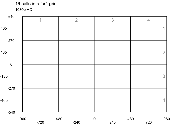
Below is the table created by the code above. Notice that there’s no 7x2 grid for 14 cells because the aspect ratio would have been too extreme, and that a single layout has been chosen for cases where there are multiple options, for example 12 cells (4x3, 6x2, etc.).
chosen_grids
## # A tibble: 8 x 10
## # Groups:   cells [8]
##    cols  rows cells width height aspect_ratio title preview_plot overlay_plot
##   <int> <int> <int> <dbl>  <dbl>        <dbl> <glu> <list>       <list>
## 1     2     2     4   960    540        1.78  4 ce… <gg>         <gg>
## 2     3     2     6   640    540        1.19  6 ce… <gg>         <gg>
## 3     4     2     8   480    540        0.889 8 ce… <gg>         <gg>
## 4     3     3     9   640    360        1.78  9 ce… <gg>         <gg>
## 5     5     2    10   384    540        0.711 10 c… <gg>         <gg>
## 6     4     3    12   480    360        1.33  12 c… <gg>         <gg>
## 7     5     3    15   384    360        1.07  15 c… <gg>         <gg>
## 8     4     4    16   480    270        1.78  16 c… <gg>         <gg>
## # … with 1 more variable: aspect_ratio_difference <dbl>
Now we’ll use the walk
function from
purrr to print each preview plot from
the table above. Unlike
map, this function
doesn’t create any output so it doesn’t print [1], [2], etc. for
each plot.
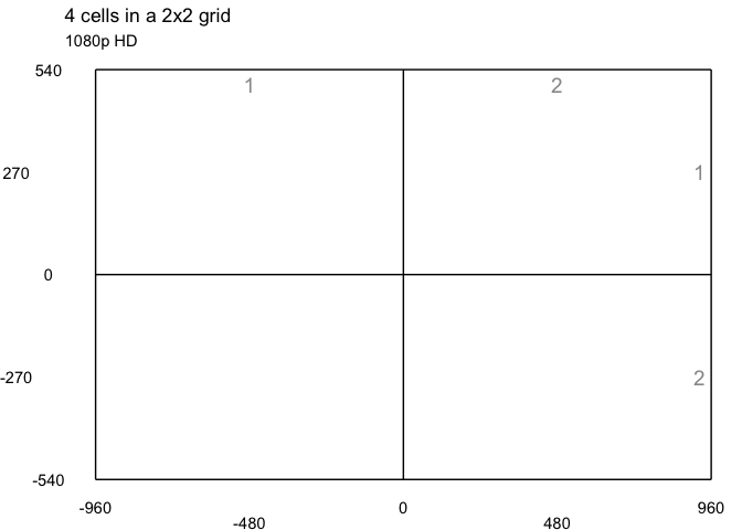
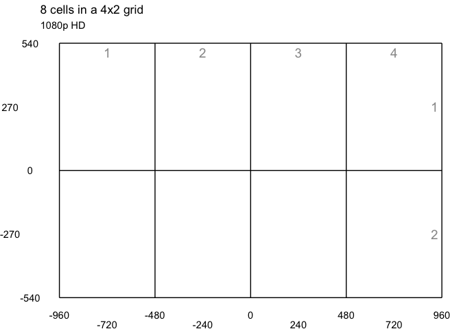
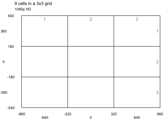
walk(chosen_grids$preview_plot, print)
We can export the overlay plots to transparent PNG files using the
ggsave function
– note the bg = "transparent" option. This time we use
walk2 to iterate
over the plots because we want to supply two arguments to ggsave: the
title of each plot and the plot itself.
walk2(
  chosen_grids$title,
  chosen_grids$overlay_plot,
  ~ ggsave(
    filename = paste0(.x, ".png"),
    plot = .y,
    path = "output",
    height = 1080/300, width = 1920/300, dpi = 300,
    bg = "transparent"
  )
)
I’ve created a ZIP file of images for 1080p grids up to 48 cells with a maximum of 8 rows or columns. You’re welcome to download this file or to modify my code above to create overlays for different grid layouts or resolutions.
If you have any questions or suggestions, why not get in touch with me on Twitter?